Next: About this document ...
Up: lab_template
Previous: lab_template
Subsections
The purpose of this lab is to use Maple to introduce you to
Taylor polynomial approximations to functions, including some
applications.
To assist you, there is a worksheet associated with this lab that
contains examples similar to some of the exercises. You can
copy that worksheet to your home directory with the following command,
which must be run in a terminal window, not in Maple.
cp /math/calclab/MA1023/Taylor_start.mws ~/My_Documents
You can copy the worksheet now, but you should read through the lab
before you load it into Maple. Once you have read through the exercises, start u
p Maple, load the worksheet, and go through it carefully. Then you can start working on the exercises.
The idea of the Taylor polynomial approximation of order  at
at
 , written
  , to a smooth function
  is to require
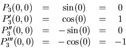
that and have the same value at .
Furthermore, their derivatives at must match up to order
. For example the Taylor polynomial of order three for
is to require
that and have the same value at .
Furthermore, their derivatives at must match up to order
. For example the Taylor polynomial of order three for  at
at
 would have to satisfy the conditions
You should check for yourself that the cubic polynomial satisfying
these four conditions is
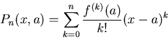
The general form of the Taylor polynomial approximation of order
to is given by the following
Theorem 1
Suppose that
is a smooth function in some open interval
containing
. Then the
th degree Taylor polynomial of the
function
at the point
is given by
We will be seeing this formula a lot, so it
would be good for you to memorize it now! The notation
 is used in the definition to stand for the value of the
 -th derivative of
  at . That is,
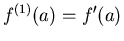 ,
,
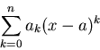
 , and so on. By convention,
 . Note that
  is fixed and so the derivatives are
just numbers. That is, a Taylor polynomial has the form
is fixed and so the derivatives are
just numbers. That is, a Taylor polynomial has the form
which you should recognize as a power series that has been truncated.
To measure how well a Taylor Polynomial approximates the function over
a specified interval ![$[c,d]$](img19.png) , we define the tolerance
, we define the tolerance  of
to be the maximum of the absolute error
of
to be the maximum of the absolute error
over the interval .
To use the Taylor and TayPlot commands you need to load the CalcP7 package.
>with(CalcP7);
The exponential function can be approximated at a base point zero with a polynomial of order four using the following command.
>Taylor(exp(x),x=0,4);
You might want to experiment with changing the order. To see
 and its fourth order polynomial use
>TayPlot(exp(x),x=0,{4},x=-4..4);
This plots the exponantial and three approximating polynomials.
>TayPlot(exp(x),x=0,{2,3,4},x=-2..2);
Notice that the further away from the base point, the further the polynomial diverges from the function. the amount the polynomial diverges i.e. its error, is simply the difference of the function and the polynomial.
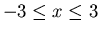
>plot(abs(exp(x)-Taylor(exp(x),x=0,3)),x=-2..2);
This plot shows that in the domain x from -2 to 2 the error around the base point is zero and the error is its greatest at x = 2 with a difference of over one. You can experiment with the polynomial orders to change the accuracy. If your work requires an error of no more than 0.2 within a given distance of the base point then you can plot your accuracy line y = 0.2 along with the difference of the function and the Taylor approximation polynomial.
>plot([0.2,abs(exp(x)-Taylor(exp(x),x=0,3))],x=-2..2,y=0..0.25);
We knew this would have some of its error well above 0.2. Change the order from three to four. As you can see there are still some values in the domain close to x = 2 whose error is above 0.2. Now try an order of 5. Is the error entirely under 0.2 between x = -2 and x = 2? Larger orders will work as well but order five is the minimum order that will keep the error under 0.2 within the given domain.
- For the following functions and base points, determine what
minimum order is required so that the Taylor polynomial approximates the
function to within a tolerance of
 over the given
interval.
over the given
interval.
-
, base point
 , interval
 ![$[-2,2]$](img25.png) .
.
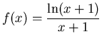
-
 , base point , interval
 ![$[-0.9,0.9]$](img27.png) .
.
-
 , base point , interval .
-
 , base point , interval .
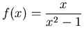
- For the function,
 , use the TayPlot command to plot the function and multiple Taylor polynomial approximations of various orders with base point on the same graph over the interval
 ; use a y-range from
  to
to  . If you increase the order of the Taylor polynomial, can you ever get a good approximation at
  ? Can you make a good guess at the radius of convergence of the Taylor series for ?
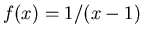
- Consider the function
 . Plot the graph of this function along with its Taylor polynomial approximation of order 4 with base point over the interval
 . Limit the
  range of your plot from
  to
to  . By increasing the order of the Taylor polynomial in your plot, can you make a good guess at the interval of convergence of the Taylor series? If you increase the order of the Taylor polynomial, can you ever get a good approximation at ?
A theorem from complex variables says that the radius of convergence of the Taylor series of a function like is the distance between the base point ( in this case) and the nearest singularity of the function. By singularity, what is meant is a value of  where the function is undefined. Where is undefined? Is the distance between this point and the base point consistent with your guess of the radius of convergence from the plot?
Next: About this document ...
Up: lab_template
Previous: lab_template
Dina Solitro
2006-02-08