Subsections

• Purpose
• Getting Started
• Background
  • Derivatives and the slope
  • Arc length
  
  
• Maple Commands
• Exercises

Parametric curves in the plane

Purpose

The purpose of this lab is to give you practice with parametric curves in the plane and in visualizing parametric curves as representing motion.

Getting Started

To assist you, there is a worksheet associated with this lab that contains examples and even solutions to some of the exercises. You can copy that worksheet to your home directory with the following command, which must be run in a terminal window, not in Maple.

cp /math/calclab/MA1023/Parametric_start_C08.mws ~/My_Documents

You can copy the worksheet now, but you should read through the lab before you load it into Maple. Once you have read to the exercises, start up Maple, load the worksheet Parametric_start_C08.mws, and go through it carefully. Then you can start working on the exercises.

Background

A parametric curve in the plane is defined as an ordered pair, $(f(t), g(t))$, of functions, with $f(t)$ representing the $x$ coordinate and $g(t)$ the $y$ coordinate. Parametric curves arise naturally as the solutions of differential equations and often represent the motion of a particle or a mechanical system. They also often arise in studying oscillations in electrical circuits.

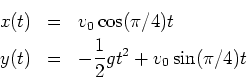
For example, neglecting air resistance, the position of a projectile fired from the origin at an initial speed of $v_0$ and angle of inclination $\pi/4$ is given by the parametric equations

$$\begin{eqnarray*} x(t) & = & v_0 \cos(\pi/4) t \\ y(t) & = & -\frac{1}{2} g t^2 + v_0 \sin(\pi/4) t \end{eqnarray*}$$

where $t$ is time and $g$ is the acceleration due to gravity.

To help you to visualize parametric curves as representing motion, a Maple routine called ParamPlot has been written. It uses the Maple animate command to actually show the particle moving along its trajectory. You actually used this command before for the lab on polar coordinates. Examples are in the Getting Started worksheet.

Derivatives and the slope

The graph of a parametric curve may not have a slope at every point on the curve. When the slope exists, it must be given by the formula from class.

$$\frac{dy}{dx} = \frac{\frac{dy}{dt}}{\frac{dx}{dt}}$$

It is clear that this formula doesn't make sense if $$\frac{dx}{dt}= 0$$ at some particular value of $t$. If $$\frac{dy}{dx} \neq 0$$ at that same value of $t$, then it turns out the graph has a vertical tangent at that point. If both $$\frac{dx}{dt}$$ and $$\frac{dy}{dt}$$ are zero at some value of $t$, then the curve often doesn't have a tangent line at that point. What you see instead is a sharp corner, called a cusp.An example of this appears in the first exercise.

Arc length

As mentioned above, parametric curves often represent the motion of a particle or mechanical system. As we will see in class, when we think of a parametric curve as representing motion, we need a way to measure the distance traveled by the particle. This distance is given by the arc length, $s$, of a curve. For a parametric curve $x=f(t)$, $y=g(t)$, the arc length of the curve for $a \leq t \leq b$ is given below.

$$s = \int_{a}^{b} \sqrt{ (f'(t))^2+(g'(t))^2} \, dt$$

While the concept of arc length is very useful for the theory of parametric curves, it turns out to be very difficult to compute in all but the simplest cases.

Maple Commands

There are a variety of ways to work with parametric equations in Maple. There is an animation command that shows how the graph is plotted over t. For example the parabola $y=x^2$ can be written parametrically in different ways two of them are $[t,t^2]$ and $[-t,t^2]$

>with(plots):
>with(CalcP7):
>implicitplot(x^2=y,x=-2..2,y=0..4,scaling=constrained);
>ParamPlot([t,t^2],t=-2..2,scaling=constrained);
>ParamPlot([-t,t^2],t=-2..2,scaling=constrained);

The ParamPlot command produces an animated plot. To see the animation, execute the command and then click on the plot region below to make the controls appear in the Context Bar just above the worksheet window. To enter a function parametrically

>f:=t->[t*cos(3*t),t^2];
>VPlot(f(t),t=-2*Pi..2*Pi);

Exercises

1. The cycloid is a famous example of a parametric curve having several important applications. Use the ParamPlot command to animate the cycloid 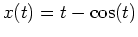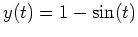$x(t) = t-\cos(t)$, $y(t) = 1-\sin(t)$ over the interval $0 \leq t \leq 6 \pi$. The sharp points in the graph are called cusps. Use the formula for the slope of a parametric curve to find values of $t$ for where these cusps occur and explain why it makes sense for the cusps to occur only at these values of $t$. That is, verify that the curve has a slope at all other values of $t$ in the interval.

2. The family of parametric curves
   
   $$( \cos(n t), \sin(m t)), \mbox{ for $0 \leq t \leq 2 \pi$},$$
   
   
   where $n$ and $m$ are positive integers, is an example of what is called a Lissajous figure. Use a parametric plot to plot the three cases $n=1,m=2$, $n=1,m=3$ and $n=3, m=1$ and describe what you see.

3. The parametric description $x=\cos(t)$, $y= 3\sin(t)$, $0 \leq t \leq 2 \pi$ is the ellipse
   
   $$x^2+ \frac{y^2}{9} = 1$$
   
   
   First show that the two are the same shape by plotting them parametrically and with the command implicitplot. Use the formula above to set up an integral for the arc length of the ellipse. You should find that Maple can't do the integral exactly. This is because this integral can't be done analytically. You can get a numerical approximation to the integral by putting an evalf command on the outside of the int command.

4. Consider the family of parametric curves $x=20\cos(t)+a\cos(bt)$ and $y=20\sin(t)+a\sin(bt)$, where $a$ and $b$ are positive constants, with $0 < a < 20$ and $b$ is a positive integer. Use a paramentric plot to test the following properties of this family.

   i

   The curve only has loops in it if $ab>20$. (Plot the example in the worksheet to see what loops look like.)

   ii

   If the curve has loops in it, the number of loops is $b-1$.

   iii

   The curve has cusps if $ab=20$ and there are exactly $b-1$ of them. Use at least two sets of values of $a$ and $b$ to test each property. Don't forget that $b$ has to be an integer and $a$ should be smaller than 20.