Next: About this document ...
Up: lab_template
Previous: lab_template
Subsections
Improper integrals like the ones we have been considering in class
have many applications, for example in thermodynamics and heat
transfer. In this lab we will consider the role of improper integrals
in probability, which also has many applications in science and
engineering.
To assist you, there is a worksheet associated with this lab that
contains examples and even solutions to some of the exercises. You can
copy that worksheet to your home directory with the following command,
which must be run in a terminal window, not in Maple.
cp /math/calclab/MA1023/Probability_start_C08.mws My_Documents
You can copy the worksheet now, but you should read through the lab
before you load it into Maple. Once you have read to the exercises,
start up Maple, load
the worksheet Probability_start.mws, and go through it
carefully. Then you can start working on the exercises.
The first concept we need is that of a random variable. Intuitively, a
random variable is used to measure an outcome whose value is not
certain. For example, the number of hours that a hard disk can run
before failing is a random variable because it is not the same for
every drive, even if we only consider identical drives from the same
production run. A few other examples of random variables that are important
in science, engineering, or manufacturing are given below.
- The time it takes for a packet of information to travel from one
location to another on the Internet.
- The number of miles that an automobile tire can be driven before
it fails.
- The lengths of supposedly identical bolts manufactured by a
particular production line.
- The speed of a particular gas molecule in a sample of a gas.
You may be more familiar with what are called discrete random
variables, for example the number of heads obtained in ten tosses of a
coin, which can only take a finite number of discrete values. In the
case of a discrete random variable, the probability of a single
outcome can be positive. For example, the probability that a single
flip of a coin produces tails is 50%. The situation is very different
when we consider a random variable like the number of miles a
tire can be driven before failure, which can take any value from
zero to something over  miles. Since there are an infinite
number of possible outcomes, the probability that the tire
fails at exactly some number of miles, for example
miles. Since there are an infinite
number of possible outcomes, the probability that the tire
fails at exactly some number of miles, for example  miles, is
zero. However, we would expect that the probability that the tire
would fail between
miles, is
zero. However, we would expect that the probability that the tire
would fail between  miles and miles would not be
zero, but would be a positive number.
miles and miles would not be
zero, but would be a positive number.
A random variable that can take on a continuous range of values is
called a continuous random variable. There turn out to be lots of
applications of continuous random variables in science, engineering,
and business, so a lot of effort has gone into devising mathematical
models. These mathematical models are all based on the following
definition.
Definition 1
We say that a random variable  is continuous if there is a function
 , called the probability density function, such that
 , for all
-
-
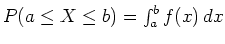 where
where
 represents the probability that the random variable is
greater than or equal to
represents the probability that the random variable is
greater than or equal to  but less than or equal to
  .
.
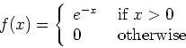
For example, consider the following function.
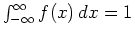
This function is non-negative, and also satisfies the second
condition, since
which is pretty easy to show. So this could be a probability density
function for a continuous random variable .
A lot of the effort involved in modeling a random process, that is, a
process whose outcome is a random variable, is in finding a suitable
probability density function. Over the years, lots of different
functions have been proposed and used. One thing that they all have in
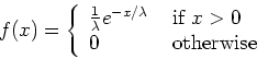
common, though, is that they depend on parameters. For example, the
general exponential probability density function is defined as
where  is a parameter that can be adjusted to get the best
fit to any particular situation.
is a parameter that can be adjusted to get the best
fit to any particular situation.
The process of deciding what probability density function to use and
how to determine the parameters is very complicated and can involve
very sophisticated mathematics. However, in the simple approach we are
taking here, the problem of determining the parameter value(s) often
depends on quantities that can be determined experimentally, for
example by collecting data on tire failure. For our purposes, the two
most important quantities are the mean,  and the standard
deviation
and the standard
deviation  . The mean is defined by
and the standard deviation is the square root of the variance,  ,
which is defined by
,
which is defined by
Probably the most important distribution is the normal distribution,
widely referred to as the bell-shaped curve. The probability density
function for a normal distribution with mean and standard
deviation is given by the following equation.
This distribution has a tremendous number of applications in science,
engineering, and business. The exercises provide a few simple ones.
In applications, one generally has to know in advance that the random
variable you want to model folows a certain kind of
distribution, at least approximately. How one would determine this is
way beyond the scope of
this course, so we won't really discuss it. On the other hand, once
you know, for example, that your random variable has a normal
distribution you only need the values of the mean and the standard
deviation to be able to model it. The exponential distribution is even
simpler, since it only has one parameter, and you only need to know
the mean of your random variable to use this distribution to model it.
One thing to keep in mind when you are using the normal distribution
as a model is that calculations can involve values of your random
variable that don't make physical sense. For example, suppose that a
machining operation produces steel shafts whose diameters have
a normal distribution, with a mean of  inches and a standard
deviation of
inches and a standard
deviation of  inch. If you were asked to compute the percentage of the
shafts in a certain production run that had diameters less than
inch. If you were asked to compute the percentage of the
shafts in a certain production run that had diameters less than  inches you would use the following integral
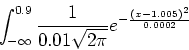
even though negative values for the shaft diameters don't make
physical sense.
- Show that the probability density function given for the
exponential distribution,
satisfies the condition
as long as is a positive number.
- Show that the mean and the standard deviation of the exponential distribution are both equal to .
- The amount of raw sugar that a sugar refinery can process in one day can be modeled as an exponential distribution with a mean of 12 tons. What is the probability that the refinery will process more than 10 tons in a single day?
- Suppose the time required to repair a car is exponentially distributed with a mean 45 minutes. What is the probability that a repair takes longer than 1 hour? Between 30 and 45 minutes?
- Suppose the time between placing an order at a fast food restaurant and receiving the order is exponentially distributed with an average wait time of 2.65 minutes. What is the probability that the customer receives their order in less than 1 minute? What is the probability that the customer waits longer than 4 minutes?
- A college professor teaches Calculus each year to a large class of first-year students. For tests, he uses standarized exams that he knows from past experience produce normal grade distributions with a mean of 76 and a standard deviation of 10. If he sets scores between 69 and 79 as the guidelines for a C, 79 to 89 for a B, and 89 or higher for an A, what percentage of the students will get A's, B's and C's in the course? Without doing any extra integral calculations, what percentage will fail?
- The average birth weight of infants in the United States is 7.8 lb, with a standard deviation of 1.1 lb. Assuming a normal distribution, what is the probability that a newborn will weigh between 6 lb and 7 lb? More than 9 lb?
Next: About this document ...
Up: lab_template
Previous: lab_template
Dina Solitro
2008-01-16