


Next: About this document ...
Up: lab_template
Previous: lab_template
Subsections
The purpose of this lab is to help you become familiar with graphs in
polar coordinates.
There are many times in math, science, and engineering that coordinate
systems other than the familiar one of Cartesian coordinates are
convenient. In this lab, we consider one of the most common and useful
such systems, that of polar coordinates.
The main reason for using polar coordinates is that they can be used
to simply describe regions in the plane that would be very difficult
to describe using Cartesian coordinates. For example, graphing the
circle  in Cartesian coordinates requires two functions -
one for the upper half and one for the lower half. In polar
coordinates, the same circle has the very simple representation
in Cartesian coordinates requires two functions -
one for the upper half and one for the lower half. In polar
coordinates, the same circle has the very simple representation  .
.
These are three types of well-known graphs in polar coordinates. The
table below will allow you to identify the graphs in the exercises.
| Name |
Equation |
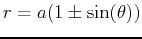
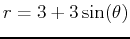
| cardioid |
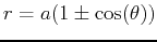 or or
 |
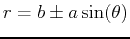
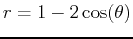
| limaçon |
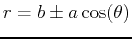 or or
 |
| rose |
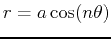 or or
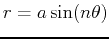 |
Finding where two graphs in Cartesian coordinates intersect is
straightforward. You just set the two functions equal and solve for
the values of  . In polar coordinates, the situation is more
difficult. Most of the difficulties are due to the following considerations.
. In polar coordinates, the situation is more
difficult. Most of the difficulties are due to the following considerations.
- A point in the plane can have more than one representation in
polar coordinates. For example, ,
 is the same
point as
is the same
point as  ,
,  . In general a point in the plane can have
an infinite number of representations in polar coordinates, just by
adding multiples of
. In general a point in the plane can have
an infinite number of representations in polar coordinates, just by
adding multiples of  to
to  . Even if you restrict
a point in the plane can have several different representations.
. Even if you restrict
a point in the plane can have several different representations.
- The origin is determined by
 . The angle can have
any value.
. The angle can have
any value.
These considerations can make finding the intersections of two graphs in polar
coordinates a difficult task. As the exercises demonstrate, it
usually requires a combination of plots and solving equations to find
all of the intersections.
>plot(cos(2*theta),theta=0..2*Pi,coords=polar);
Don't forget the option ,coords=polar!
This graph is a four-leafed rose. Polar graphs can be hard to understand. Animating the graph as the angle increases will help.
>with(CalcP7):
>ParamPlot([cos(2*t),t],t=0..2*Pi,coords=polar);
When you run the ParamPlot command, you first get a set of axes with no curves drawn, and you think that there is something wrong. What you need to do to see the curves is first click on the graph. A box appears around the graph and a set of controls appears in the context bar just below the menu shortcut buttons at the top of the main Maple window. The set of controls works like those on a VCR. To see the animated graph, click on the play button. The other controls in the context bar allow you to slow down or speed up the animation, step through the animation one frame at a time, stop the animation, and even run the animation in reverse. I suggest you play with them until you feel comfortable.
To find where two graphs intersect you set the functions equal to each other as they both equal the radius and then solve for the angle.
>plot([1+cos(theta),3/2],theta=0..2*Pi,coords=polar);
>plot([1+cos(theta),3/2],theta=0..2*Pi);
As discussed above there can be infinite solutions so use the fsolve command and choose a range of angles values in which the intersection point occurs.
>t1:=fsolve(1+cos(theta)=3/2,theta=0..2);
>t2:=fsolve(1+cos(theta)=3/2,theta=4..6);
The following commands find the radius vaue for each angle.
>1+cos(t1);
>1+cos(t2);
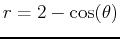
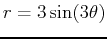
- For each of the following polar equations, plot the graph in polar coordinates using the plot command and identify the graph as a
cardioid, limaçon, or rose.
- A)
-

- B)
-
- C)
-
- Find all points of intersection for each pair of curves in polar
coordinates.
- A)
-
 and
and
 for
for
 .
.
- B)
-
and
 for
.
for
.
- The equation of a rose is
 . For two consecutive integer values of
  ,
find the domain necessary to trace one full petal of the rose, plot the petal and find its area. Then, find the area of the entire rose.
,
find the domain necessary to trace one full petal of the rose, plot the petal and find its area. Then, find the area of the entire rose.
Next: About this document ...
Up: lab_template
Previous: lab_template
Dina J. Solitro-Rassias
2018-02-22