In mathematics, the function that takes a real number as input and
returns its integer part is called the greatest integer
function. The notation used is  and the formal definition is that
 is the largest integer n satisfying
  . Another common
name for this function is the floor function,
. Another common
name for this function is the floor function,  , and
that is the name used by Maple. See the examples below.
, and
that is the name used by Maple. See the examples below.
> floor(21/4);

> floor(13.543);

> plot(floor(x),x=0..4);
> plot(floor(x),x=0..10);
Next, consider the plot generated by the following Maple command.
> plot(x-floor(x),x=0..4);
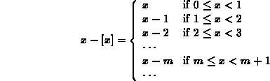
To help you understand the plot, recall that if  , then
 so
so  . Now, if
  then
then  so
so 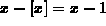 . In fact,
we could describe
. In fact,
we could describe  with the following formula
There is one thing to watch out for, though. Compare the plots generated by the following commands.
> plot(x-floor(x),x=0..8);
> plot(x-floor(x),x=0..8,numpoints=1000);
The first plot generated is not an accurate plot of  . You can
tell this because the peaks are not at the same height, as they should
be. The second command uses the numpoints parameter to tell
Maple to plot more points. There is nothing special about the value
1000, however, you should just increase the value of this parameter
until you get a plot that looks right.
. You can
tell this because the peaks are not at the same height, as they should
be. The second command uses the numpoints parameter to tell
Maple to plot more points. There is nothing special about the value
1000, however, you should just increase the value of this parameter
until you get a plot that looks right.
Now, suppose that L is a positive real number and consider the following expression.

You should be able to convince yourself that the following formula holds.
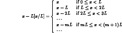
You can try the following Maple commands if you need more help
visualizing how  behaves.
> plot(x-2*floor(x/2),x=0..4);
> plot(x-6*floor(x/6),x=0..24,numpoints=250);
Notice how the value of L affects not only the interval at which the graph repeats, but also the maximum value attained.
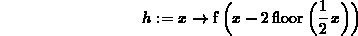
Finally, suppose we have a function  and we define a new function
 by
by

After a little thought, you should be able to convince yourself that

for any value of x. This means that the function  only depends
on the values of
only depends
on the values of  for
for  . In fact the graph of
 for
for  consists of copies of the graph of
  for
for  translated to the right by multiples of L.
As an example, consider the function
translated to the right by multiples of L.
As an example, consider the function  . Try the following
Maple commands.
. Try the following
Maple commands.
> f := x -> x^2+1;

> g := x -> f(x-floor(x));

> plot(g(x),x=0..5,numpoints=200);
> h := x -> f(x-2*floor(x/2));
> plot(h(x),x=0..5);
> h3 := x -> f(x-3*floor(x/3));

> plot(h3(x),x=0..6);