Subsections

• Purpose
• Background
  • Partial derivatives
  
  
• Tangent Lines and Planes
• Exercises

Partial Derivatives and their Geometric Interpretation

Purpose

The purpose of this lab is to acquaint you with using Maple to compute partial derivatives.

Background

For a function $f(x)$ of a single real variable, the derivative $f'(x)$ gives information on whether the graph of $f$ is increasing or decreasing. Finding where the derivative is zero was important in finding extreme values. For a function $F(x,y)$ of two (or more) variables, the situation is more complicated.

Partial derivatives

A differentiable function, $F(x,y)$, of two variables has two partial derivatives: $\partial F /\partial x$ and $\partial F /\partial y$. As you have learned in class, computing partial derivatives is very much like computing regular derivatives. The main difference is that when you are computing $\partial F /\partial x$, you must treat the variable $y$ as if it was a constant and vice-versa when computing $\partial F /\partial y$.

The Maple commands for computing partial derivatives are D and diff. The diff command can be used on both expressions and functions whereas the D command can be used only on functions. The examples below show all first order and second order partials in Maple.

> f := (x,y) -> x^2*y^2-x*y;
> diff(f(x,y),x);
> diff(f(x,y),y);
> diff(f(x,y),x,x);
> diff(f(x,y),y,y);
> diff(f(x,y),x,y);
> D[1](f)(x,y);
> D[2](f)(x,y);
> D[1,1](f)(x,y);
> D[2,2](f)(x,y);
> D[1,2](f)(x,y);

The next example shows how to evaluate the mixed partial derivative of the function given above at the point $(-1,1)$.

> der := diff(f(x,y),x,y);
> subs({x=-1,y=1},der);
> D[1,2](f)(-1,1);

Tangent Lines and Planes

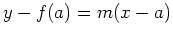The tangent plane like the tangent line to a single variable function is based on derivatives, however the partial derivatives are used for the tangent plane. Let's start with the equation of the tangent line to the function $f(x)$ at the point where $x=a$. Recall, the general equation of a line at the point $(a,f(a)$ having slope $m$ is $y-f(a) = m(x-a)$. This can be rewritten knowing that the derivative is the slope of a tangent line as 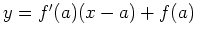$y = f'(a)(x-a) + f(a)$. Similarly for a funcion of two variables, the equation of the plane tangent to $z=f(x,y)$ at the point $(a,b)$ has the equation 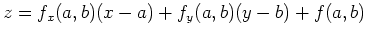$$z = f_x(a,b)(x-a)+f_y(a,b)(y-b)+f(a,b)$$. The following example will show you how this can easily be translated to Maple syntax.

> g := x-> sin(x)-x^3/7+x^2;
> tanline := D(g)(5)*(x-5)+g(5);
> plot({g(x),tanline},x=-2..8);

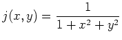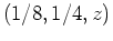The next example shows how to find the tangent plane to the function $$j(x,y)=\frac{1}{1+x^2+y^2}$$ at $(1/8,1/4,z)$. You could write the partials with diff or D. This example uses D as it is easier to plug in the the point with this syntax; with diff the subs command would be used.

> f:=(x,y)->1/(1+x^2+y^2);
> tp:=D[1](f)(1/8,1/4)*(x-1/8)+D[2](f)(1/8,1/4)*(y-1/4)+f(1/8,1/4);
> plot3d({f(x,y),tp},x=-1..1,y=-1..1,style=patchnogrid);

To find a point where the tangent plane is horizontal, you would need to solve where both first order partials are equal to zero simultaneously.

> solve({diff(f(x,y),x)=0,diff(f(x,y),y)=0},{x,y});

Exercises

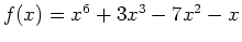
1. Given the single variable function $f(x)=x^6+3x^3-7x^2-x$

   a)

   Plot $f(x)$ over the interval $-2 \leq x \leq 2$.

   b)

   Find the slope of $f$ at $x=1$.

   c)

   Find another $x$ value that has the same slope as the slope at $x=1$.

   d)

   Find the slope of the line containing the $x$ values from parts b and c.

   e)

   Find the equation of a single line that is tangent to the graph of $f(x)$ at both points from parts b and c snf plot the function and the tangent line on the same graph over the interval given in part a to show the line is tangent at both points.

2. Given:
   
   $$h(x,y)=2x \cos(y) - y \sin(x)$$
   
   

   a)

   Find the tangent plane at $(-2,3,z)$.

   b)

   Plot the function $h(x,y)$ and the tangent plane over the intervals $-4 \leq x \leq 0$ and $1 \leq y \leq 5$ and rotate the plot so that you can see that the plane is tangent.

3. There is only one point at which the plane tangent to the surface $z=x^2+xy+2y^2-5x+8y$ is horizontal. Find it and plot it along with the function on the same graph. Be sure to use axes so that you can rotate the graph and see that the tangent plane is horizontal.