Subsections

• Getting Started
• Background
  • Contour lines
  • Directional derivatives
  • The Gradient
  
  
• Exercises

MA 1024 Lab 4: Contour lines, directional derivatives, and the gradient

Getting Started

To assist you, there is a worksheet associated with this lab that contains examples. You can copy that worksheet to your home directory with the following command, which must be run in a terminal window, not in Maple.

cp /math/calclab/MA1024/Pardiff_grad_start.mws ~

You can copy the worksheet now, but you should read through the lab before you load it into Maple. Once you have read to the exercises, start up Maple, load the worksheet Pardiff_grad_start.mws, and go through it carefully. Then you can start working on the exercises.

Background

Contour lines

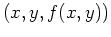The graph of a function of a single real variable is a set of points $(x,f(x))$ in the plane. Typically, the graph of such a function is a curve. For functions of two variables in Cartesian coordinates, the graph is a set of points $(x,y,f(x,y))$ in three-dimensional space. For this reason, visualizing functions of two variables is usually more difficult. For stude nts, it is usually even more difficult if the surface is described in terms of polar or spherical coordinates.

One of the most valuable services provided by computer software such as Maple is that it allows us to produce intricate graphs with a minimum of effort on our part. This becomes especially apparent when i t comes to functions of two variables, because there are many more comp utations required to produce one graph, yet Maple performs all these com putations with only a little guidance from the user. The simplest way of describing a surface in Cartesian coordinates is as the graph of a function $z=f(x,y)$ over a domain, e.g. a set of points in the $xy$ plane. The domain can have any shape, but a rectangular one is the easiest to deal with. Another way of representing a surface $z=f(x,y)$ is through the use of level curves. The idea is that a plane $z=c$ intersects the surface in a curve. The projection of this curve on the $xy$ plane is called a level curve. A collection of such curves for different values of $c$ is a representation of the surface called a contour plot.

Directional derivatives

The partial derivatives $\partial F /\partial x$ and $\partial F /\partial y$ of $F$ can be thought of as the rate of change of $F$ in the direction parallel to the $x$ and $y$ axes, respectively. The directional derivative $D_{\mathbf{u}}F(\mathbf{p})$, where $\mathbf{u}$ is a unit vector, is the rate of change of $F$ in the direction $\mathbf{u}$. There are several different ways that the directional derivative can be computed. The method most often used for hand calculation relies on the gradient, which will be described below. It is also possible to simply use the definition

$$D_{\mathbf{u}}F(\mathbf{p}) = \lim_{h \rightarrow 0} \frac{F(\mathbf{p}+h\mathbf{u}) - F(\mathbf{p})}{h}$$

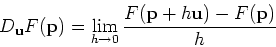
to compute the directional derivative. However, the following computation, based on the definition, is often simpler to use.

$$D_{\mathbf{u}}F(\mathbf{p}) = \left. \frac{d}{dt} F(\mathbf{p}+t\mathbf{u}) \, \right\vert _{t=0}$$

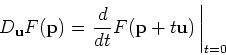
One way to think about this that can be helpful in understanding directional derivatives is to realize that $\mathbf{p}+t\mathbf{u}$ is a straight line in the $x,y$ plane. The plane perpendicular to the $x,y$ plane that contains this straight line intersects the surface $z = F(x,y)$ in a curve whose $z$ coordinate is $F(\mathbf{p}+t\mathbf{u})$. The derivative of $F(\mathbf{p}+t\mathbf{u})$ at $t=0$ is the rate of change of $F$ at the point $\mathbf{p}$ moving in the direction $\mathbf{u}$.

Maple doesn't have a simple command for computing directional derivatives. There is a command in the tensor package that can be used, but it is a little confusing unless you know something about tensors. Fortunately, the method described above and the method using the gradient described below are both easy to implement in Maple. Examples are given in the Getting Started worksheet.

The Gradient

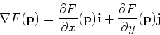
The gradient of $F$, written $\nabla F$, is most easily computed as

$$\nabla F(\mathbf{p}) = \frac{\partial F}{\partial x}(\mathbf{... ...thbf{i} + \frac{\partial F}{\partial y}(\mathbf{p}) \mathbf{j}$$

As described in the text, the gradient has several important properties, including the following.

• The gradient can be used to compute the directional derivative as follows.
  
  $$D_{\mathbf{u}}F(\mathbf{p}) = \nabla F(\mathbf{p}) \cdot \mathbf{u}$$
  
  

• The gradient $\nabla F(\mathbf{p})$ points in the direction of maximum increase of the value of $F$ at $\mathbf{p}$.
• The gradient $\nabla F(\mathbf{p})$ is perpendicular to the level curve of $F$ that passes through the point $\mathbf{p}$.
• The gradient can be easily generalized to apply to functions of three or more variables.

Maple has a fairly simple command grad in the linalg package (which we used for curve computations). Examples of computing gradients, using the gradient to compute directional derivatives, and plotting the gradient field are all in the Getting Started worksheet.

Exercises

1. Consider the following function.
   
   $$f(x,y) = \frac{x-y+1}{1+x^2+y^2}$$
   
   

   A)

   First, plot the graph of this function over the domain $-3 \leq x \leq 3$ and $-3 \leq y \leq 3$ using the plot3d command. Then use the contourplot command to generate a contour plot of $f$ over the same domain having 20 contour lines.

   B)

   What does the contour plot look like in the regions where the surface plot has a steep incline? What does it look like where the surface plot is almost flat?

   C)

   What can you say about the surface plot in a region whe re the contour plot looks like a series of nested circles?

2. Consider the function from exercise 1 which looks like a valley with a mountain opposite it. Is it p ossible to find a path from the point $$(-2,-3)$$ to $$(3,2)$$ such that the valu e of $z$ is always between $-0.25$ and $0.25$ ? You do not have to find a formula for your path, but you must present convincing evi dence that it exists. For example, you might want to sketch your p ath in by hand on an appropriate countour plot.

3. Consider again the function $f$ from the first exercise. Using either method from the Getting Started worksheet, compute the directional derivative of $f$ at the point $x=1$, $y= -1$ in the three directions below.

   A)

   $\mathbf{u} = \langle 1, 1 \rangle$

   B)

   $\mathbf{u} = \langle 1, 0 \rangle$

   C)

   $\mathbf{u} = \langle 0, 1 \rangle$

4. Using the method from the Getting Started worksheet, plot the gradient field and the contours of $f$ on the same plot. Use the domain of $0 \leq x \leq 3$ and $-3 \leq y \leq 0$. Can you use this plot to explain the values for the directional derivatives you obtained in the previous exercises? By explaining the values, I only mean can you explain what kind of surface it is and why the values were positive, negative, or zero in terms of the contours and the gradient field?