Subsections

• Introduction
• Entering an expression
• Entering a function
• Evaluating functions and expressions
• Solving a function or an expression algebraically
• Solving a function or an expression numerically
• Some more strange output
• Defining and plotting 3D explicit functions and implicit equations
• Exercises

Assigning Labels and Solving Equations with Maple

Introduction

The purpose of this lab is to learn the basic commands needed in any Maple lab.

Entering an expression

Expressions such as $x^3+3x^2-x+1$ can be entered in a similar way to variable assignment. Choose a variable name to represent the expression and assign the expression to the variable as follows.

> expr := x^3+3*x^2-x+1;

Entering a function

Suppose you want to enter the same expression stored in expr above, but as a function of $x$. In Maple, you would type

> f := x-> x^2+2*x-6;

Below is how NOT to enter a function:

> f(x) := x^2+2*x-6;

The difference between expressions and functions are first the obvious, that expressions do not have to satisfy the definition of a function in the sense that for each input $x$, there is a unique value $f(x)$. A function may be defined as an expression, but not all expressions can be defined as functions. The differences in Maple are numerous as you will see below when we evaluate the expression or function for a given value as well as when using the plot command.

Evaluating functions and expressions

In order to evaluate an expression at a given value of $x$, you must use the subs or eval command. For example, if we wanted to evaluate the expression expr$=x^3+3x^2-x+1$ at $x=2$, the example below show how this can be done

> subs(x=2,expr);
> eval(expr,x=2);
> r:=sin(theta) + 8*theta^2;
> subs(theta=Pi/2,r);

In the subs command, the first argument tells Maple what you would like to substitute in for $x$. The second argument tells Maple what expression you are substituting into. Note the difference in outputs when a whole number or fraction is entered compared to a decimal.

>g:=2*x/3;
>subs(x=4,g);
>eval(g,x=1/2);
>subs(x=4.0,g);

The evalf command is used when we want Maple to output the answer in decimal form. If this command is not used, the output to your Maple commands will be calculated analytically, where as the evalf command forces Maple to calculate the answers numerically. The evalf command has one essential argument, however a second argument can be added in order to tell how many digits we want to be in the answer as shown below. >evalf(eval(expr,x=Pi)); >evalf(eval(expr,x=Pi),20); In Maple, functions are much easier to evaluate than expressions. In order to evaluate the function $f(x)=x^3+3x^2-x+1$ at $x=2$, simply type

> f(2);

Solving a function or an expression algebraically

You can set an expression or function equal to another expression, function, or number inside a solve command.As an example, you may want to find where the following two parabolas intersect.

> g := 9*x^2-14;
> h:=-x^2;
> plot([g,h],x=-2..2);
> solve(g=h,x);

The plot shows that there are two intersection points and the solve command finds both $x$ values.It is good to get into the habit of naming your output so you can use it in a later command. Giving the $x$ values a name makes it easy to plug them into the function to find the $y$ values.

> ip:=solve(g=h,x);

Since there are two $x$ values called $ip$, use [ ] to call up the one you want.

> eval(g,x=ip[1]);
> eval(h,x=ip[2]);

Therefore the two intersection points are $(\frac{\sqrt{35}}{5},\frac{-7}{5})$ and $(\frac{-\sqrt{35}}{5},\frac{-7}{5})$. This seems like the answer shown on the graph.

Solving a function or an expression numerically

If you would like to find where the following function crosses the horizontal line $y=-50$ you can try the solve command.

> j:=x->2*x^3-15*x^2-2*x+5;
> k:=x->-50;
> plot([j(x),k(x)],x=-3..8);

The graph shows there should be three answers.

> solve(j(x)=k(x),x);

That is some scary output! So instead of using the algebraic solve try the numerical fsolve.

> fsolve(j(x)=k(x),x);

Some more strange output

If you want to find where the following function crosses the x-axis, just set it equal to zero.

> f:=theta->-1/2*theta+sin(theta);
> plot(f(theta),theta=-8*Pi..8*Pi);
> solve(f(theta)=0,theta);

Wow, what is that?!?! We know from the graph that there should be three answers and solve wasn't a great option so try fsolve again.

> fsolve(f(theta)=0,theta);

Where are the other two answers!? This is actually how fsolve usually works. It shoots for one answer and only gives that one. But you can tell fsolve where to look by getting an idea from the graph and typing that domain into the fsolve command.

> a:=fsolve(f(theta)=0,theta=-5..-1);
> b:=fsolve(f(theta)=0,theta=-1..1);
> c:=fsolve(f(theta)=0,theta=1..5);

To find the $y$ values just plug in the names of the $x$ values.

> f(a);
> f(b);
> f(c);

(Of course the y-values are zero!)

Defining and plotting 3D explicit functions and implicit equations

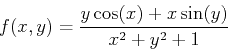
If $z$ is explicitly defined as a function of $x$ and $y$, you can use function notation and generate a surface plot using Maple's plot3d command. If $z$ is not explicitly solved for and assumed to be a function of $x$ and $y$, the implicit equation can be defined as an expression and you can generate a surface plot using Maple's implicitplot3d command. A few examples are shown below.

> with(plots):
> f:=(x,y)->x^2+y^2;
> plot3d(f(x,y),x=-5..5,y=-5..5);
> f(2,1);
> surf:=x^2+y^2+z^2=9;
> with(plots):
> implicitplot3d(surf,x=-5..5,y=-5..5,z=-5..5);
> solve(eval(surf,{x=2,y=1}),z);

Exercises

1. Given the expression $$4x^6-\frac{20}{3}x^5+\frac{88}{3}x^4-\frac{160}{3}x^3-\frac{172}{3}x^2+60x+24$$,

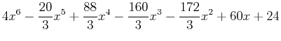   A)

   Plot the expression and in text state how many roots it has. That is, how many times the it crosses the x-axis.(Experiment with domain values until you find values that show the crossing points clearly.)

   B)

   Compare outputs from the Maple solve and fsolve command to find the $x$ values of where it crosses the x-axis. State the real roots in text.

   C)

   Use the Maple eval command to verify at least one of the roots to show it is zero.

2. Given the functions 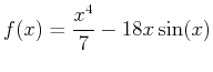$$f(x)=\frac{x^4}{7}-18x\sin(x)$$ and $$h(x)=1.8x-10$$

   A)

   Plot the functions. Again experiment with domain values until the intersection points are clear. Then state in text how many intersection points you see.

   B)

   Compare outputs from the Maple solve and fsolve command to find all $x$ values where the two functions intersect. Label the $x$ values with a variable in front of the solve or fsolve command.

   C)

   Find all corresponding $y$ values and state the intersection points in text.(When writing your text sentence use 3 significant figures for the answer. Be sure to round properly!)

3. Plot each of the 3-D surfaces given below using -5 to 5 for all plotting ranges and find the corresponding $z$ value at the point $(1,-3)$.

   A)

   
   

   $$f(x,y)=\frac{y\cos(x)+x\sin(y)}{x^2+y^2+1}$$

   
   

   B)

   
   

   $$\frac{x^2}{2}-\frac{y^2}{2}+z^2=-1$$