Next: About this document ...
Up: lab_template
Previous: lab_template
Subsections
The purpose of this lab is to acquaint you with using Maple to compute
partial derivatives, directional derivatives, and the gradient.
To assist you, there is a worksheet associated with this lab. You can copy that worksheet to your home directory by copying the directory location below to your computer's Start menu search or in your Maple screen, go to File - Open, then paste the dirctory location in the dialogue box where it says file name.
\\storage.wpi.edu\academics\math\calclab\MA1024\Pardiff_grad_start_A19.mw
For a function  of a single real variable, the derivative
 gives information on whether the graph of
  is increasing or
decreasing. Finding where the derivative is zero was important in
finding extreme values. For a function
is increasing or
decreasing. Finding where the derivative is zero was important in
finding extreme values. For a function  of two (or more)
variables, the situation is more complicated.
of two (or more)
variables, the situation is more complicated.
A differentiable function, , of two variables has two partial
derivatives:
 and
and
 . As you have learned in class, computing partial derivatives is
very much like computing regular derivatives. The main difference is
that when you are computing
, you must treat
the variable
. As you have learned in class, computing partial derivatives is
very much like computing regular derivatives. The main difference is
that when you are computing
, you must treat
the variable  as if it was a constant and vice-versa when computing
.
as if it was a constant and vice-versa when computing
.
The Maple commands for computing partial derivatives are D
and diff. The diff command can be used on both expressions and functions whereas the D command can be used only on functions. The commands below show examples of first order and second order partials in Maple.
> f := (x,y) -> x^2*y^2-x*y;
> diff(f(x,y),x);
> diff(f(x,y),y,y);
> D[1](f)(x,y);
> D[2,2](f)(x,y);
Note in the above D command that the 1 in the square brackets means x and the 2 means y.
The next example shows how to evaluate the mixed partial derivative of the function given above at the point
 .
.
> eval(diff(f(x,y),x,y),{x=-1,y=1});
> D[1,2](f)(-1,1);
The partial derivatives
and
of  can be thought of as the rate of change of in
the direction parallel to the
can be thought of as the rate of change of in
the direction parallel to the  and axes, respectively. The
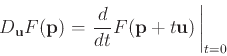
directional derivative
and axes, respectively. The
directional derivative
 , where
 is a unit vector, is the rate of change of in the
direction . There are several different ways that the
directional derivative can be computed. The method most often used
for hand calculation relies on the gradient, which will be described
below. It is also possible to simply use the definition
is a unit vector, is the rate of change of in the
direction . There are several different ways that the
directional derivative can be computed. The method most often used
for hand calculation relies on the gradient, which will be described
below. It is also possible to simply use the definition
to compute the directional derivative. However, the following
computation, based on the definition, is often simpler to use.
One way to think about this that can be helpful in understanding
directional derivatives is to realize that
 is
a straight line in the
is
a straight line in the  plane. The plane perpendicular to the
plane that contains this straight line intersects the surface
plane. The plane perpendicular to the
plane that contains this straight line intersects the surface  in a curve whose
  coordinate is
 . The derivative of
at
. The derivative of
at  is the rate of change of at
the point
is the rate of change of at
the point  moving in the direction .
Maple doesn't have a simple command for computing directional
derivatives. There is a command in the tensor package that
can be used, but it is a little confusing unless you know something
about tensors. Fortunately, the method described above and the method
using the gradient described below are both easy to implement in
Maple. Examples are given in the Getting Started worksheet.
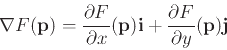
The gradient of , written  , is most easily computed as
As described in the text, the gradient has several important
properties, including the following.
Maple has a fairly simple command grad in the linalg
package (which we used for curve computations). Examples of computing
gradients, using the gradient to compute directional derivatives, and
plotting the gradient field are all in the Getting Started
worksheet.
- Use partial derivatives in Maple to answer each of the following:
- a)
- A function is called harmonic if it satisfies Laplaces equation
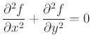 . Which of the functions below are harmonic?
-
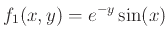
-
-
- b)
- What is the relationship between
 and
and  for which
 would satisfy the one-dimensional heat equation
 . Substitute and with that relationship and show that the heat equation is satisfied.
- For the function
 ,
,
- a)
- Compute the directional derivative of at the point
 in each of the directions below. Explain what your results tell about the surface at that point in the given direction in terms of being positive, negative or zero. Be sure to use a unit vector in your calculation of the directional derivative.
-
-

-
- b)
- Plot the gradient field of over the intervals
 and
and
 using a
 ![$[10,10]$](img41.png) grid and fieldstrength=fixed and plot each direction vector from above at the point
on the same plot. Based on the relationship between the direction vector and the gradient, explain why the directional derivatives above were positive, negative or zero.
grid and fieldstrength=fixed and plot each direction vector from above at the point
on the same plot. Based on the relationship between the direction vector and the gradient, explain why the directional derivatives above were positive, negative or zero.
- c)
- Copy and paste ONLY the fieldplot from the previous exercise. Delete the colon and change the plotting intervals to
 and
and
 with a
 ![$[20,20]$](img44.png) grid and fieldstrength=fixed. Given what you know about the relationship between gradient vectors and direction of greates rate of change, can you estimate the
grid and fieldstrength=fixed. Given what you know about the relationship between gradient vectors and direction of greates rate of change, can you estimate the  ordered pair where may have a local maximum?
Next: About this document ...
Up: lab_template
Previous: lab_template
Dina J. Solitro-Rassias
2019-09-03