Subsections

• Purpose
• Background
  • Partial derivatives
  • The gradient
  • Directional derivatives
  • Tangent planes and linear approximations
• Exercises

Partial derivatives, directional derivatives, gradients, and tangent planes

Purpose

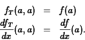
The purpose of this lab is to acquaint you with differentiating multivariable functions.

Background

Partial derivatives

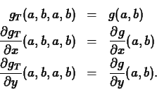
You are already familiar with the Maple D and diff commands for computing derivatives. These same commands can be used to compute partial derivatives. As you have already learned, the diff command is for differentiating Maple expressions and the D command operates on functions. Examples are given below.

First, we define an expression.

  > 
p := x^2*sin(x*y);

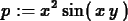
These commands compute $\frac{\partial p}{\partial x}$ and $\frac{\partial p}{\partial y}$.

  > 
diff(p,x);

  > 
diff(p,y);

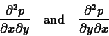
Higher order deriviatives are specified just by adding more arguments. The following commands compute the mixed partial derivatives

$$\frac{\partial^2 p}{\partial x \partial y}\quad\hbox{and}\quad \frac{\partial^2 p}{\partial y \partial x}$$

  > 
diff(p,x,y);

  > 
diff(p,y,x);

The D command can be simpler to use in some cases. However, it only works on functions and you have to remember that the output of the D command is also a function. Here are some examples.

  > 
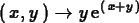
f := (x,y) -> y*exp(x+y);

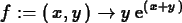
Here is $\frac{\partial f}{\partial x}$ computed using the diff command:

  > 
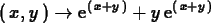
diff(f(x,y),x);

And the same thing using the D command:

  > 
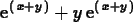
D[1](f);

Here is the command for $\frac{\partial f}{\partial y}$

  > 
D[2](f);

When you define a function of two or more variables in Maple, you always have to provide names for the independent variables, and order is important. In the case of the function $f$ we defined above, $x$ is the first independent variable and $y$ is the second. The D command uses this order to specify partial derivatives. For example, to find

$$\frac{\partial^2 f}{\partial x^2}$$

the syntax for the D command is as follows.

  > 
D[1,1](f);

To obtain

$$\frac{\partial^2 f}{\partial x \partial y}$$

use the following command.

  > 
D[1,2](f);

To obtain the expression corresponding to a partial derivative rather than the function, use the following syntax. You can also use this syntax to evaluate a partial derivative at a specific point.

  > 
D[1,2](f)(x,y);

  > 
D[1,2](f)(0,1);

The gradient

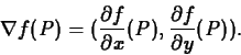
Definition 1   Suppose that $f(x,y)$ is differentiable at a point $P$ (see the text). Then the gradient of $f$, denoted $\nabla f(P)$, is the vector

$$\nabla f(P) = (\frac{\partial f}{\partial x}(P),\frac{\partial f}{\partial y}(P)).$$

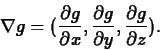
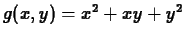
For example, if 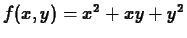$f(x,y)=x^2+xy+y^2$, then

$$\nabla f = (2x+y,x+2y).$$

In Maple, you can calculate gradients using the grad command in the linalg package.

  > 
with(linalg):

Warning: new definition for   norm
Warning: new definition for   trace

  > 
g := (x,y) -> x^2+x*y+y^2;

  > 
del_g := grad(g(x,y),[x,y]);

Note that the argument of grad is an expression and the output is also an expression. Unfortunately, there is no elegant way to use the output of grad as a function. The easiest way to evaluate the gradient at a specific point is as follows:

  > 
subs(x=3,y=1,evalm(del_g));

The evalm command is necessary when substituting into vectors. See what happens without it.

The definition is straightforward to generalize to functions of three or more independent variables - you just have as many components as the number of independent variables. That is, for $g(x,y,z)$ you would have

$$\nabla g = (\frac{\partial g}{\partial x},\frac{\partial g}{\partial y},\frac{\partial g}{\partial z}).$$

The Maple command for the gradient extends to this situation as well.

Directional derivatives

We know that $\frac{\partial f}{\partial x}$ is the instantaneous rate of change of $f$ in the direction of the unit vector ${\bf i}$ and that, similarly, $\frac{\partial f}{\partial y}$ is the instantaneous rate of change of $f$ in the direction of the unit vector ${\bf j}$. The gradient can be used to find the instantaneous rate of change in other directions as follows.

Definition 2   Suppose that $f(x,y)$ is differentiable at a point $P$. Then for an arbitrary unit vector ${\bf u}$, the directional derivative of $f$ at $P$ in the direction ${\bf u}$, denoted $D_{\bf u}f(P)$ is

$$D_{\bf u}f(P) = \nabla f(P) \cdot {\bf u}.$$

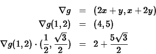
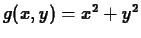
For example, let $g(x,y)=x^2+xy+y^2$, $P = (1,2)$ and ${\bf u} = (\frac{1}{2}, \frac{\sqrt{3}}{2})$. Then we have

$$\begin{eqnarray*} \nabla g & = & (2x+y,x+2y) \\ \nabla g(1,2) & = & (4,5) \\ \... ...(\frac{1}{2}, \frac{\sqrt{3}}{2}) & = & 2 + \frac{5 \sqrt{3}}{2} \end{eqnarray*}$$

In Maple, computing directional derivatives can be a little clumsy, because of the difficulties in substituting into the gradient. One way to calculate a directional derivative is shown below.

  > 
with(linalg):

Warning: new definition for   norm
Warning: new definition for   trace

  > 
g := (x,y) -> x^2+x*y+y^2;

  > 
del_g := grad(g(x,y),[x,y]);

  > 
u := vector([1/2,sqrt(3)/2]);

  > 
r := subs({x=1,y=2},evalm(del_g));

Again, note the evalm command.

  > 
innerprod(r,u);

Tangent planes and linear approximations

When we studied the calculus of functions of a single variable, we used the derivative of a function $f(x)$ at a specific point $x=a$ to construct the linear approximation, $f_T(x,a)$, given by the equation

$$f_T(x,a) = f^{\prime} (a)\ast (x-a) + f(a).$$

In the case of a function from $\mathbf{R}^n$ to $\mathbf{R}$, $n \geq 2$, we clearly have to do something different because we have more than one independent variable. As we will see below, it turns out that the linear approximation is a function that is linear in each of the independent variables. Thus, in the case of a function $g(x,y)$, we would expect the linear approximation at a point $(a,b)$, denoted $g_T(x,y,a,b)$ to have the form

$$g_T(x,y,a,b) = Ax + By + C$$

which is the equation of a plane. Recall that the linear approximation of a scalar function satisfied the two conditions

$$\begin{eqnarray*} f_T(a,a) & = & f(a) \\ \frac{df_T}{dx}(a,a) & = & \frac{df}{dx}(a). \end{eqnarray*}$$

By analogy, you might expect the linear approximation to $g(x,y)$ at a point $(a,b)$ to satisfy the conditions

$$\begin{eqnarray*} g_T(a,b,a,b) & = & g(a,b) \\ \frac{\partial g_T}{\partial x}(... ...}{\partial y}(a,b,a,b) & = & \frac{\partial g}{\partial y}(a,b). \end{eqnarray*}$$

These turn out to be the correct conditions, and lead to the formula

$$g_T(x,y,a,b) = g(a,b) +\frac{\partial g}{\partial x}(a,b)\ast(x-a) + \frac{\partial g}{\partial y}(a,b)\ast(y-b).$$ (1)

A Maple procedure called TanPlane is available in the CalcP package. TanPlane outputs an expression that can be plotted or otherwise manipulated. For example, you might want to plot it together with the original function as shown below.

  > 
with(CalcP):

  > 
h := (x,y) -> x^2+y^2+2;

  > 
TanPlane(h(x,y),x=1,y=2);

  > 
plot3d({h(x,y),TanPlane(h(x,y),x=1,y=2)},x=-5..5,y=-5..5);

Exercises

1. Compute the first and second order partial derivatives of the function
   
   $$f(x,y) = \exp(-x)\cos(y^2)$$
   
   
   Use Maple to plot the function and its first order partial derivatives (not on the same plot).

2. In the previous lab, you learned how to use the contourplot command. Can you use a contour plot of a function to obtain information about the gradient of the function? Illustrate your answer by providing a contour plot of a function of your own choosing on which you have drawn arrows at three points that represent the gradient.

3. Find the equations of the tangent planes for the following functions at the specified points. Plot the graph of the function and the tangent plane on the same plot. Be sure to choose a viewpoint and a domain that best illustrates the relationship between the function and the tangent plane.
   1. $g(x,y) = x^2+y^2$ at $(1,-1)$.
   2. $g(x,y) = \cos(2x)\sin(y)$ at $(\pi/2,\pi/4)$.
   3. $g(x,y) = \exp(x) y$ at $(0,1)$.

4. Is there a way to use the tangent plane at a specific point to compute the directional derivative at that same point? Show at least one example to illustrate your answer.