Subsections

• Purpose
• Getting Started
• Background
  • Least Squares
  
  
• Exercises

MA 1024: Least Squares Method of Approximation

Purpose

The purpose of this lab is to acquaint you with the application of local extreme values as it applies to the method of least-squares.

Getting Started

To assist you, there is a worksheet associated with this lab that contains examples. You can copy that worksheet to your home directory with the following command, which must be run in a terminal window, not in Maple.

cp /math/calclab/MA1024/Least_squares_start_B08.mws My_Documents

You can copy the worksheet now, but you should read through the lab before you load it into Maple. Once you have read to the exercises, start up Maple, load the worksheet Least_squares_start_B08.mws, and go through it carefully. Then you can start working on the exercises.

Background

Many applications of calculus involve finding the maximum and minimum values of functions. For example, suppose that there is a network of electrical power generating stations, each with its own cost for producing power, with the cost per unit of power at each station changing with the amount of power it generates. An important problem for the network operators is to determine how much power each station should generate to minimize the total cost of generating a given amount of power.

A crucial first step in solving such problems is being able to find and classify local extreme values of a function. What we mean by a function $f$ having a local extreme value at a point $\mathbf{p}_0$ is that for values of $\mathbf{p}$ near $\mathbf{p}_0$, $f(\mathbf{p}_0) \geq f(\mathbf{p})$ for a local maximum and $f(\mathbf{p}_0) \leq f(\mathbf{p})$ for a local minimum.

In single-variable calculus, we found that we could locate candidates for local extreme values by finding points where the first derivative vanishes. For functions of two dimensions, the condition is that both first order partial derivatives must vanish at a local extreme value candidate point. Such a point is called a stationary point. It is also one of the three types of points called critical points. Note carefully that the condition does not say that a point where the partial derivatives vanish must be a local extreme point. Rather, it says that stationary points are candidates for local extrema. Just as was the case for functions of a single variable, there can be stationary points that are not extrema. For example, the saddle surface 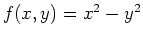$f(x,y) = x^2-y^2$ has a stationary point at the origin, but it is not a local extremum.

Finding and classifying the local extreme values of a function $f(x,y)$ requires several steps. First, the partial derivatives must be computed. Then the stationary points must be solved for, which is not always a simple task.

$$\frac{\partial f}{\partial x}=0=\frac{\partial f}{\partial y}$$

Next, one must check for the presence of singular points, which might also be local extreme values. Finally, each critical point must be classified as a local maximum, local minimum, or neither using the second-partials test

If $f_{xx}(a,b)f_{yy}(a,b)-[f_{xy}(a,b)]^2 >0$ and $f_{xx}(a,b) > 0$ then $f(a,b)$ is a local minimum.
If $f_{xx}(a,b)f_{yy}(a,b)-[f_{xy}(a,b)]^2 >0$ and $f_{xx}(a,b) < 0$ then $f(a,b)$ is a local maximum.
If $f_{xx}(a,b)f_{yy}(a,b)-[f_{xy}(a,b)]^2 <0$ then $f(a,b)$ is a saddle point.
If $f_{xx}(a,b)f_{yy}(a,b)-[f_{xy}(a,b)]^2 =0$ then no conclusion can be made.

Least Squares

The least-squares method is based on the linear equation $y=ax+b$. Given data points, this method finds the equation of the line closest to all the data points. It does this by finding an a and b value such that the vertical distance to the least-squares line is a minimum. When the sum of all the distances squared is minimized, the result yields a slope and y-intercept of the line that best fits the data.

$$f(a,b)=d_{1}^2+d_{2}^2+...+d_{n}^2=\sum_{i=1}^n[y_{i}-(ax_{i}+b)]^2$$

Notice that the function to be minimized is a function of two variables and therefore the second-partials test will be used. The linear equation is not always the best fit for every set of data. We will look at a few other types of non-linear functions. One example is the power law $$y = Ax^{\alpha}$$. Taking the natural log of both sides gives us a linear relationship between $\ln x$ and $\ln y$ as follows:

$$\ln y = \ln A + \alpha \ln x$$

Another example is the exponential function $$y=A e^{\alpha x}$$ which again after taking the natural log of both sides results in a linear relationship between $x$ and $\ln y$ as follows:

$$\ln y = \ln A + \alpha x$$

Exercises

Given the data below, use the first column as data values for $x$.

X	Y1	Y2	Y3
1	11.3	8.04	1.81
2	6.94	19.5	1.38
3	5.70	17.4	1.49
4	12.1	20.7	1.34
5	6.95	30.5	0.802
6	20.4	23.1	0.901
7	14.6	76.8	0.985
8	17.9	60.6	1.46
9	26	81.2	0.828
10	22.8	97.6	0.844
11	22.9	114	0.727
12	25.3	129	0.639
13	31	150	0.698
14	33.7	148	0.531
15	31.4	190	0.0482
16	34.2	193	0.510
17	25.5	212	0.378
18	38.7	225	0.471
19	38	247	0.292
20	44.9	270	0.360

1. Use the second column as data values for $y$. Plot the data set $(x_i,y_i)$. Find the least-squares line that best fits the data and then plot the data set along with the least-squares line.
2. Use the third column as data values for $y$. Plot the data set $(x_i,y_i)$. Find a power-law function that best fits the data. Include a plot of the data set the corresponds to $(\ln x_i,\ln y_i)$ along with the least-squares line and also a plot of the original data set $(x_i,y_i)$ along with the power-law function that best fits the data.
3. Use the fourth column as data values for $y$. Plot the data set $(x_i,y_i)$. Find an exponential funtion that best fits the data. Include a plot of the data set the corresponds to $(x_i,\ln y_i)$ along with the least-squares line and also a plot of the original data set $(x_i,y_i)$ along with the exponential function that best fits the data.