Next: About this document ...
Up: lab_template
Previous: lab_template
Subsections
The purpose of this lab is to acquaint you with using Maple to compute
partial derivatives, directional derivatives, and the gradient.
To assist you, there is a worksheet associated with this lab that
contains examples. You can
copy that worksheet to your home directory with the following command,
which must be run in a terminal window, not in Maple.
cp /math/calclab/MA1024/Pardiff_grad_start_C11.mw My_Documents
Another way to access the getting started worksheet is to go to your computer's Start menu and choose run. In the run field type:
\\filer\calclab
when you hit enter, you can then choose MA1024 and then choose the worksheet Pardiff_grad_start_C11.mw
Remember to immediately save it in your home directory. Once you've copied and saved the worksheet, read through the background on the internet and the backgr ound of the worksheet before starting the exercises.
For a function  of a single real variable, the derivative
 gives information on whether the graph of
  is increasing or
decreasing. Finding where the derivative is zero was important in
finding extreme values. For a function
is increasing or
decreasing. Finding where the derivative is zero was important in
finding extreme values. For a function  of two (or more)
variables, the situation is more complicated.
of two (or more)
variables, the situation is more complicated.
A differentiable function, , of two variables has two partial
derivatives:
 and
and
 . As you have learned in class, computing partial derivatives is
very much like computing regular derivatives. The main difference is
that when you are computing
, you must treat
the variable
. As you have learned in class, computing partial derivatives is
very much like computing regular derivatives. The main difference is
that when you are computing
, you must treat
the variable  as if it was a constant and vice-versa when computing
.
as if it was a constant and vice-versa when computing
.
The Maple commands for computing partial derivatives are D
and diff. The Getting Started worksheet has examples
of how to use these commands to compute partial derivatives.
The partial derivatives
and
of  can be thought of as the rate of change of in
the direction parallel to the
can be thought of as the rate of change of in
the direction parallel to the  and axes, respectively. The
directional derivative
and axes, respectively. The
directional derivative
 , where
 is a unit vector, is the rate of change of in the
direction . There are several different ways that the
directional derivative can be computed. The method most often used
for hand calculation relies on the gradient, which will be described
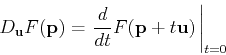
below. It is also possible to simply use the definition
is a unit vector, is the rate of change of in the
direction . There are several different ways that the
directional derivative can be computed. The method most often used
for hand calculation relies on the gradient, which will be described
below. It is also possible to simply use the definition
to compute the directional derivative. However, the following
computation, based on the definition, is often simpler to use.
One way to think about this that can be helpful in understanding
directional derivatives is to realize that
 is
a straight line in the
is
a straight line in the  plane. The plane perpendicular to the
plane that contains this straight line intersects the surface
plane. The plane perpendicular to the
plane that contains this straight line intersects the surface  in a curve whose
  coordinate is
 . The derivative of
at
. The derivative of
at  is the rate of change of at
the point
is the rate of change of at
the point  moving in the direction .
Maple doesn't have a simple command for computing directional
derivatives. There is a command in the tensor package that
can be used, but it is a little confusing unless you know something
about tensors. Fortunately, the method described above and the method
using the gradient described below are both easy to implement in
Maple. Examples are given in the Getting Started worksheet.
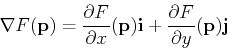
The gradient of , written  , is most easily computed as
As described in the text, the gradient has several important
properties, including the following.
Maple has a fairly simple command grad in the linalg
package (which we used for curve computations). Examples of computing
gradients, using the gradient to compute directional derivatives, and
plotting the gradient field are all in the Getting Started
worksheet.
- For the function
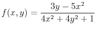 ,
,
- A)
- Generate a contourplot of over the domain
 and
and
 .
.
- B)
- Compute the two first order partial derivatives of at the point
 .
.
- C)
- If you were standing on the surface of at the point , would you be standing on a hill or in a valley?
- Using method 2 from the Getting Started worksheet, compute the directional derivative of at the points ,
 and
and  in each of the directions below. What do your results suggest about the surface at these points? What is different about the zero answer for the point compared to the other two points?
-
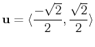
-
- Using the method from the Getting Started worksheet, plot the gradient field and the contours of on the same plot over the intervals
 and
and
 . Use 30 contours, a
 ![$[20,20]$](img35.png) grid and fieldstrength=fixed for the gradient plot. Describe the surface of at the points and using both the gradient field and the countour plot in your explanation.
grid and fieldstrength=fixed for the gradient plot. Describe the surface of at the points and using both the gradient field and the countour plot in your explanation.
Next: About this document ...
Up: lab_template
Previous: lab_template
Dina J. Solitro-Rassias
2011-01-31