Next: About this document ...
Up: lab_template
Previous: lab_template
Subsections
The purpose of this lab is to acquaint you with using Maple to compute
partial derivatives, directional derivatives, and the gradient.
To assist you, there is a worksheet associated with this lab that
contains examples and even solutions to some of the exercises. You can
copy that worksheet to your home directory by going to your computer's Start menu and choose run. In the run field type:
\\filer\calclab
when you hit enter, you can then choose MA1024 and then choose the worksheet
Pardiff_grad_start_C13.mw
Remember to immediately save it in your own home directory. Once you've copied and saved the worksheet, read through the background on the internet and the background of the worksheet before starting the exercises.
For a function  of a single real variable, the derivative
 gives information on whether the graph of
  is increasing or
decreasing. Finding where the derivative is zero was important in
finding extreme values. For a function
is increasing or
decreasing. Finding where the derivative is zero was important in
finding extreme values. For a function  of two (or more)
variables, the situation is more complicated.
of two (or more)
variables, the situation is more complicated.
A differentiable function, , of two variables has two partial
derivatives:
 and
and
 . As you have learned in class, computing partial derivatives is
very much like computing regular derivatives. The main difference is
that when you are computing
, you must treat
the variable
. As you have learned in class, computing partial derivatives is
very much like computing regular derivatives. The main difference is
that when you are computing
, you must treat
the variable  as if it was a constant and vice-versa when computing
.
as if it was a constant and vice-versa when computing
.
The Maple commands for computing partial derivatives are D
and diff. The Getting Started worksheet has examples
of how to use these commands to compute partial derivatives.
Many applications of calculus involve finding the maximum and minimum values of functions. For example, suppose that there is a network of electrical power generating stations, each with its own cost for producing power, with the cost per unit of power at each station changing with the amount of power it generates. An important problem for the network operators is to determine how much power each station should generate to minimize the total cost of generating a given amount of power.
A crucial first step in solving such problems is being able to find and classify local extreme values of a function. What we mean by a function having a local extreme value at a point  is that for values of
  near ,
 for a local maximum and
 for a local minimum.
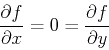
In single-variable calculus, we found that we could locate candidates for local extreme values by finding points where the first derivative vanishes. For functions of two variables, the condition is that both first order partial derivatives must vanish at a local extreme value candidate point. Such a point is called a stationary point. It is also one of the three types of points called critical points. Note carefully that the condition does not say that a point where the partial derivatives vanish must be a local extreme point. Rather, it says that stationary points are candidates for local extrema. Just as was the case for functions of a single variable, there can be stationary points that are not extrema. For example, the saddle surface
 has a stationary point at the origin, but it is not a local extremum.
Finding and classifying the stationary points of a function  requires several steps. First, the partial derivatives must be computed. Then the stationary points must be solved for by solving where both partial derivatives equal zero simultaneously.
Next, one must check for the presence of singular points, which might also be local extreme values. Finally, each critical point must be classified as a local maximum, local minimum, or a saddle point using the second-partials test:
If
![$f_{xx}(x_0,y_0)f_{yy}(x_0,y_0)-[f_{xy}(x_0,y_0)]^2 >0 $](img15.png) and
and
 then
then  is a local minimum.
If
and
 then is a local maximum.
If
![$f_{xx}(x_0,y_0)f_{yy}(x_0,y_0)-[f_{xy}(x_0,y_0)]^2 <0$](img19.png) then is a saddle point.
then is a saddle point.
If
![$f_{xx}(x_0,y_0)f_{yy}(x_0,y_0)-[f_{xy}(x_0,y_0)]^2 =0$](img20.png) then no conclusion can be made. The examples in the Getting Started worksheet are intended to help you learn how to use Maple to simplify these tasks.
then no conclusion can be made. The examples in the Getting Started worksheet are intended to help you learn how to use Maple to simplify these tasks.
The partial derivatives
and
of  can be thought of as the rate of change of in
the direction parallel to the
can be thought of as the rate of change of in
the direction parallel to the  and axes, respectively. The
directional derivative
and axes, respectively. The
directional derivative
 , where
 is a unit vector, is the rate of change of in the
direction . There are several different ways that the
directional derivative can be computed. The method most often used
for hand calculation relies on the gradient, which will be described
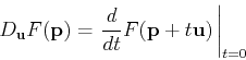
below. It is also possible to simply use the definition
is a unit vector, is the rate of change of in the
direction . There are several different ways that the
directional derivative can be computed. The method most often used
for hand calculation relies on the gradient, which will be described
below. It is also possible to simply use the definition
to compute the directional derivative. However, the following
computation, based on the definition, is often simpler to use.
One way to think about this that can be helpful in understanding
directional derivatives is to realize that
 is
a straight line in the
is
a straight line in the  plane. The plane perpendicular to the
plane that contains this straight line intersects the surface
plane. The plane perpendicular to the
plane that contains this straight line intersects the surface  in a curve whose
  coordinate is
 . The derivative of
at
. The derivative of
at  is the rate of change of at
the point moving in the direction .
is the rate of change of at
the point moving in the direction .
Maple doesn't have a simple command for computing directional
derivatives. There is a command in the tensor package that
can be used, but it is a little confusing unless you know something
about tensors. Fortunately, the method described above and the method
using the gradient described below are both easy to implement in
Maple. Examples are given in the Getting Started worksheet.
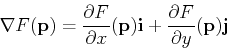
The gradient of , written  , is most easily computed as
As described in the text, the gradient has several important
properties, including the following.
Maple has a fairly simple command grad in the linalg
package (which we used for curve computations). Examples of computing
gradients, using the gradient to compute directional derivatives, and
plotting the gradient field are all in the Getting Started
worksheet.
For the function
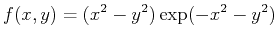 ,
,
- Using the method from the Getting Started worksheet, compute the directional derivative of at the point
 in each of the directions below. Explain your results in terms of being positive, negative or zero and what that tells about the surface at that point in the given direction.
-
-

-

- Repeat the above exercise using only the first two directions and the points
 ,
,  and
and  . What do your results suggest about the surface at these points?
- Find and classify the stationary points for using the second derivative test.
- Using the method from the Getting Started worksheet, plot the gradient field and the contours of on the same plot over the intervals
 and
and
 . Use 30 contours, a
 ![$[30,30]$](img47.png) grid and fieldstrength=fixed for the gradient plot. Describe how this plot supports your answer in the previous exercise using both the gradient field and the countour plot in your explanation.
grid and fieldstrength=fixed for the gradient plot. Describe how this plot supports your answer in the previous exercise using both the gradient field and the countour plot in your explanation.
Next: About this document ...
Up: lab_template
Previous: lab_template
Dina J. Solitro-Rassias
2013-02-05