Next: About this document ...
Up: lab_template
Previous: lab_template
Subsections
The purpose of this lab is to acquaint you with techniques for finding global extreme values of functions of two variables.
Many applications of calculus involve finding the maximum and minimum
values of functions. For example, suppose that there is a network of
electrical power generating stations, each with its own cost for
producing power, with the cost per unit of power at each station
changing with the amount of power it generates. An important problem
for the network operators
is to determine how much power each station should generate to
minimize the total cost of generating a given amount of power.
A crucial first step in solving such problems is being able to find
and classify local extreme values of a function. What we mean by a
function  having a local extreme value at a point
  is
that for values of
is
that for values of  near ,
 for a local maximum and
 for a local minimum.
In one-dimensional calculus, the absolute or global extreme values of
a function occur either at a point where the derivative is zero, a
boundary point, or where the derivative fails to exist. The situation
for a function of two variables is very similar, but the problem is
much more difficult because the boundary now consists of curves
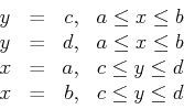
instead of just endpoints of intervals. For example, suppose that we
wanted to find the global extreme values of a function  on the
rectangle
on the
rectangle
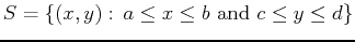 . The boundary of this rectangle consists of the four line
segments given below.
. The boundary of this rectangle consists of the four line
segments given below.
The basic theorem on the existence of global maximum and minimum values is
the following.
Theorem 1
Suppose is continuous on a closed, bounded set  , then
attains its absolute
maximum value at some point
, then
attains its absolute
maximum value at some point  in and absolute minimum value at
some point
in and absolute minimum value at
some point  in .
in .
This theorem only says that the extrema exist, but doesn't help at all
in finding them. However, we know that the global extrema occur either
at local extrema, on the boundary of the region, or at points where
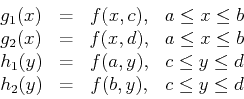
one or the other partial derivative fails to exist. For example, to
find the extreme values of a
function on the rectangle given above, you would first have to
find the interior critical points and then find the extreme values for
the four one-dimensional functions
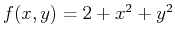
In order to find the absolute (or global) extrema given the paraboloid
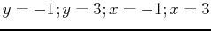
 whose domain is the rectangle made of the four lines
 , first enter the three-dimensional function.
>f:=(x,y)->2+x^2+y^2;
Keep your work organized; you may want to work your way through dimensions. Starting with the three dimensional function find the critical points by setting both partials equal to zero; you can do this in one command line. (Notice that there are no undefined points)
>solve({diff(f(x,y),x)=0,diff(f(x,y),y)=0},{x,y});
Next find the critical points along the two-dimensional domain which is the rectangular boundary.The trick is to replace one of the variables with part of the boundary.Since there are four 2-d functions (or sides) this will be done four times.
>solve(diff(f(-1,y),y)=0);
>solve(diff(f(3,y),y)=0);
>solve(diff(f(x,-1),x)=0);
>solve(diff(f(x,3),x)=0);
This gives us the four points
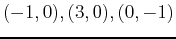 , and
, and  . Now the one-dimensional domain is simply the corners:
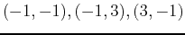 , and
, and  . Now that you have all possible points listed you simply need to plug them all into the original function to find the nine z-values. One point plugged into is shown below. The highest and lowest will be the absolute maximum and absolute minimum.
>evalf(f(-1,0))
- Find the global extrema of
over the region bounded by the rectangle
 ,
,
 .
.
- Find the global extrema of
over the elliptical region  bounded by
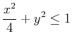 .
.
Next: About this document ...
Up: lab_template
Previous: lab_template
Dina J. Solitro-Rassias
2018-02-06