Subsections

• Purpose
• Getting Started
• Background
• Partial derivatives
• The tangent plane for explicitly defined surfaces
• The tangent plane for implicitly defined surfaces
• Exercises

Partial Derivatives and the Tangent Plane

Purpose

The purpose of this lab is to acquaint you with applications using Maple to compute partial derivatives.

Getting Started

To assist you, there is a worksheet associated with this lab. You can copy that worksheet to your home directory by copying the directory location below to your computer's Start menu search or in your Maple screen, go to File - Open, then paste the dirctory location in the dialogue box where it says file name.

\\storage.wpi.edu\academics\math\calclab\MA1024\Pardiff_tanplane_start_D19.mw

Background

When differentiating a function $$F(x,y)$$ of two (or more) variables, you need to specify which independent variable is being derived.

Partial derivatives

A differentiable function, $$F(x,y)$$, of two variables has two first order partial derivatives: $$\partial F /\partial x$$ and $$\partial F /\partial y$$. As you have learned in class, computing partial derivatives is very much like computing regular derivatives. The main difference is that when you are computing $$\partial F /\partial x$$, you must treat the variable $y$ as if it was a constant and vice-versa when computing $$\partial F /\partial y$$.

The Maple commands for computing partial derivatives are D and diff. The diff command can be used on both expressions and functions whereas the D command can be used only on functions. The commands below show examples of first order and second order partials in Maple.

> f := (x,y) -> x^2*y^2-x*y;
> diff(f(x,y),x);
> diff(f(x,y),y,y);
> D[1](f)(x,y);
> D[2,2](f)(x,y);

Note in the above D command that the 1 in the square brackets means x and the 2 means y. The next example shows how to evaluate the mixed partial derivative of the function given above at the point $$(-1,1)$$.

> eval(diff(f(x,y),x,y),{x=-1,y=1});
> D[1,2](f)(-1,1);

The tangent plane for explicitly defined surfaces

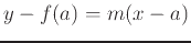The tangent plane like the tangent line to a single variable function is based on derivatives, however the partial derivatives are used for the tangent plane. Let's start with the equation of the tangent line to the function $$f(x)$$ at the point where $$x=a$$. Recall, the general equation of a line at the point $$(a,f(a)$$ having slope $$m$$ is $$y-f(a) = m(x-a)$$. This can be rewritten knowing that the derivative is the slope of a tangent line as 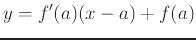$$y = f'(a)(x-a) + f(a)$$. Similarly for a funcion of two variables, the equation of the plane tangent to $z=f(x,y)$ at the point $(a,b)$ has the equation 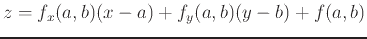$$z = f_x(a,b)(x-a)+f_y(a,b)(y-b)+f(a,b)$$. The following examples will show you how to find the tangent plane to the function 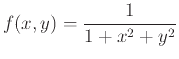$$f(x,y)=\frac{1}{1+x^2+y^2}$$ at $$(\frac{1}{8},\frac{1}{4})$$. You could write the partials with diff or D. This example uses D as it is easier to plug in the the point with this syntax; with diff, the eval or subs command would be used.

> f:=(x,y)->1/(1+x^2+y^2);
> tp:=D[1](f)(1/8,1/4)*(x-1/8)+D[2](f)(1/8,1/4)*(y-1/4)+f(1/8,1/4);
> plot3d({f(x,y),tp},x=-1..1,y=-1..1);

To find a point, $$(x_0,y_0)$$, where the tangent plane is horizontal, you would need to solve where both first order partials are equal to zero simultaneously.

> solve({diff(f(x,y),x)=0,diff(f(x,y),y)=0},{x,y});

The horizontal plane at that point would simply be $$z=f(x_0,y_0)$$. Since the solve command above yields the $(x,y)$ ordered pair $(0,0)$, below is how to plot the surface and the horizontal tangent plane.

> tp:=f(0,0);
> plot3d({f(x,y),tp},x=-1..1,y=-1..1);

The tangent plane for implicitly defined surfaces

If $z$ is not explicitly solved for but assumed to be a function of $$x$$ and $$y$$, then the equation can be defined implicitly. Note the difference in the syntax for defining the surface for the implicitplot command. An equal sign must be included in the equation and defined as an expression, not a function. This gives the flexibility of being able to graph equations without having to solve for $$z$$ first.

>with(plots):
>surf:=x^2+y^2+z^2=1;
>implicitplot3d(surf,x=-2..2,y=-2..2,z=-2..2);

The tangent plane to an implicitly defined surface $$F(x,y,z)=0$$ is given below:

$$F_x(x_0,y_0,z_0)(x-x_0)+F_y(x_0,y_0,z_0)(y-y_0)+F_z(x_0,y_0,z_0)(z-z_0)=0$$

To find the tangent plane to the sphere $$x^2+y^2+z^2=1$$ at the point $$(\frac{1}{2},-\frac{1}{2})$$ and $$z$$ is positive, you would first need to find the coordinating $$z$$ value for the $$(x,y)$$ ordered pair. Below is how you would do this in Maple as well as find and plot the tangent plane implicitly.

>with(plots):
>F:=x^2+y^2+z^2-1;
>solve(eval(F,{x=1/2,y=-1/2}),z);
>a:=eval(diff(F,x),{x=1/2,y=-1/2,z=sqrt(2)/2});
>b:=eval(diff(F,y),{x=1/2,y=-1/2,z=sqrt(2)/2});
>c:=eval(diff(F,z),{x=1/2,y=-1/2,z=sqrt(2)/2});
>tp:=a*(x-1/2)+b*(y+1/2)+c*(z-sqrt(2)/2)=0;
>implicitplot3d({F=0,tp},x=-2..2,y=-2..2,z=-2..2,numpoints=2000);

Exercises

1. Given
   
   $$f(x,y) = \frac{x+y}{1+2x^2+2y^2}$$
   
   

   a)

   Find the equation of the plane tangent to the surface $f(x,y)$ at $(-\frac{1}{3},-\frac{1}{4})$. Plot the surface and the tangent plane on the same graph over the intervals $-1 \leq x \leq 1$, $-1 \leq y \leq 1$ and rotate to see point of tangency.

   b)

   Find all points on the graph of $f(x,y)$ where the tangent plane is horizontal, then find the equation of each horizontal plane and plot them on the same graph as the function $f(x,y)$. Use plotting ranges $-3 \leq x \leq 3$, $-3 \leq y \leq 3$.

2. a)

   Use implicit methods to find the plane(s) tangent to the ellipsoid
   

   $$\frac{(x-1)^2}{3}+\frac{(y+1)^2}{2}+z^2=1$$

   
   

   at the point $(2,-1)$. Plot the tangent plane(s) on the same graph as the ellipsoid and rotate to see the point of tangency. Use plotting ranges $-1 \leq x \leq 3$, $-3 \leq y \leq 2$, and $-2 \leq z \leq 2$.

   b)

   Find all points on the ellipsoid where the tangent plane is horizontal, then find the equation of each horizontal plane and plot them on the same graph using the same plotting ranges given in part a.

3. Define the total differential from the linearization of
   
   $$u(x,y)=(-\frac{\cos^2(x)}{2}+\frac{1}{4}(\cos^2(y)\sin^2(x)+\sin^2(y)\cos^2(x))e^{-\frac{y}{x}}$$
   
   
   and estimate the change in u given small changes in $x$ and $y$ of $dx=0.1$ and $dy=0.2$ respectively at each of the following points:

   a)

   $(1,2)$

   b)

   $(0.001,0.001)$

   c)

   $$(\frac{\pi}{2},\frac{\pi}{2})$$

   Compare these answers to the actual total differential and explain these results in terms of the fieldplot of $u$ over the intervals $-2 \leq x \leq 2$, $-2 \leq y \leq 2$.