Purpose
The purpose of this lab is to give you practice using Maple to plot and animate graphs of vector functions, to compute curvature, and to specify the graphs' shapes.

Background
As we've seen in class, computing the curvature, , and the unit normal and tangent vectors is a tedious process, even for the simplest of curves. Fortunately, Maple procedures can be written to do these calculations and this lab will introduce you to the ones that we have written here at WPI as part of the CalcP package. Before you can use any of these commands, you must load the package with the following command. Since some of the commands use the linalg package, it is probably a good idea to load it as well.

> with(linalg):
Warning, new definition for norm
Warning, new definition for trace
> with(CalcP):

VDiff

Differentiates vector-valued functions

VPlot

Plots vector-valued functions in two and three dimensions

VMag

Computes the magnitude of a vector

ParamPlot

Animates parametric curves in two dimensions

ParamPlot3D

Animates parametric curves in three dimensions

Speed

Computes the speed of a particle moving on a path defined by a vector-valued function r(t)

unitvect

Computes the unit vector associated with a vector v

tanvect

Computes the unit tangent vector, T(t), for a vector-valued function r(t)

normalvect

Computes the unit normal vector, N(t), for a vector-valued function r(t)

Curvature

Computes the curvature, (t), for a vector-valued function r(t)

Examples
For more examples, see the help screens for the individual procedures. Note that all of the procedures accept either Maple vectors or Maple lists as arguments. Note also that several of the procedures allow you to evaluate the result at a specific value of t by using a second argument of the form t=a (to evaluate at t=a). If the second argument is simply t, then the result of the procedure is an expression involving t. This does not apply to the VDiff command, however, where argumets after the first are used to indicate derivatives.

  > circ := t -> vector([12*sin(t),12*cos(t)]);

  > VDiff(circ(t),t);

  > tanvect(circ(t),t);

  > normalvect(circ(t),t);

  > Curvature(circ(t),t);

  > r := t -> vector([t,t^2]);

  > tanvect(r(t),t);

  > tanvect(r(t),t=0);

  > tanvect(r(t),t=1);

Computing the unit normal vector is always more complicated than computing the unit tangent vector . In addition, Maple likes to do computations as generally as possible, which can cause complications. In particular, Maple assumes that all variables can be complex numbers. This isn't a good assumption in calculus, so the tanvect, normalvect, and Curvature procedures had to be written to give results that are real numbers. A side-effect of this is that results of the commands, especially the normalvect command, do not always appear in the simplest form. Consider the following example.

  > normalvect(r(t),t);

The notation appears because Maple had to differentiate the absolute value function to obtain the normal vector. Recall that the deriviative of is 1 if x > 0 and -1 if x < 0. Maple's notation stands for the derivative of , evaluated at . Because Maple assumes that t can be complex, it allows for to be negative. In our calculations, can never be negative so the value of is simply 1.

This may seem like a pain, but it won't affect your ability to compute normal vectors at fixed values of t, as shown in the following examples, or plot normal vectors. Putting the absolute value in several of the CalcP package functions for curve comptations was a necessary evil, because leaving it out produced answers that were just plain wrong. By putting it in, the procedures give the correct answer, but in a form that is more complicated than we would like.

  > normalvect(r(t),t=0);

  > normalvect(r(t),t=1);

  > Curvature(r(t),t);

The absolute value also appears in the output of the Curvature procedure, as shown above. This means that if you differentiate the output of the Curvature function, for example to find extreme values, you may see the Maple abs procedure in the results. You shouldn't be alarmed by this, just remember that the value will always be 1. Fortunately, the Maple solve command usually handles cases involving the abs procedure just fine.

In the following example, plots of a vector-valued function and its curvature are generated. You should compare the two plots and try to understand their relationships.

  > plot(Curvature(r(t),t),t=-2..2);

  > VPlot(r(t),t=-2..2);

The next few commands deal with a simple example of a curve known as a helix.

  > h := t -> vector([cos(t),sin(t),t]);

  > VPlot(h(t),t=0..4*Pi);

  > ParamPlot3D(h(t),t=0..4*Pi);

  > tanvect(h(t),t);

  > Speed(h(t),t);

  > Curvature(h(t),t);

  > normalvect(h(t),t);

More Examples
These commands will show you how to find a line tangent to a vector valued function at a given point, then graph both on the same plot.

> with(CalcP): with(linalg):
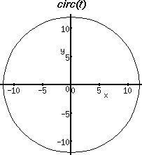
> circ := t -> vector([12*sin(t), 12*cos(t)]);

You may use options to include more information on your plots, or to make it easier to read. Use accents (not single quotes) to designate a string for a title.

> VPlot(circ(t), t=0..2*Pi, color=RED, axes=NORMAL, labels=[x,y], title=`circ(t)`);

This command will find the tangent vector at a given point, but it will not give you a tangent line.

> slope:= tanvect(circ(t),t=Pi/3);

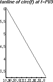
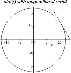
Maple's tangentline command does not work for vector valued functions, so you need to make the line yourself. Here is a relatively painless way to do this. Basically tanline is of the form slope*t + c, where c is the point of tangency (here circ(t) evaluated at t=Pi/3). Note that tanline is simply an expression, not a function. You should not type tanline(t). You can arbitrarily choose your interval for the plot of tanline to make it longer or shorter. Try -Pi..Pi for example.

> tanline:= evalm((scalarmul(slope,t)) + circ(Pi/3));

In order to display both plots on the same graph, you need to store the instructions for plotting into a variable, then use the plots[display] command.

> VPlotcirc:=VPlot(circ(t), t=0..2*Pi, color=RED, axes=NORMAL, labels=[x,y], title=`circ(t) with tangentline at t=Pi/3`):
> VPlottanline:=VPlot(tanline, t=-2*Pi..2*Pi, color=YELLOW):
> plots[display]([VPlotcirc,VPlottanline]);

For 3D graphs, you should use the right mouse button to rotate or pivot the image for a clearer view. Use the middle mouse key to redisplay. To compare two 3D graphs, you should rotate them all into the same position. If, after rotating, you notice the scaling is different, you may want to try Projection(Constrained) on the VPlot menu bar, in order to get an accurate comparison. Also, choose a type of axes for reference e.g. Normal.

Exercises
1.   A particle's position vector at time t is determined by

R(t) = 2i + 2j + 2k + (cos t) i -  j  + (sin t) i +  j +  k .

(i)		Plot and animate the graph of R(t).
(ii)		Given the animated picture, do you think this graph is substantially three-dimensional or does it all lie in a plane?
(iii)		If you feel the curve is planar, try to specify its plane. To this end, consider an arbitrary point of the curve, say, the point R(0) = 2i + 2j + 2k + i - j, and attempt to find a constant vector n such that [R(t) - R(0)] · n = 0     for all t.
(iv)		Find the curvature of the graph at the points t = 0, t = /4, and t = /2.
(v)		On the basis of (iv), can you make a plausible hypothesis about the genuine shape of the graph?
(vi)		If your answer to (v) is "yes", please specify your point and give a detailed description of the curve.

2.   Explore graphically the behavior of the helix

R(t) = (cos at)i + (sin at)j + btk

as you change the values of the constants a and b.

Set b=1. Plot the helix R(t) together with the tangent line to the curve at t=3/2 for a = 1, 2, and 4 over the interval 0<=t<=4. Describe in your own words what happens to the graph of the helix and the position of the tangent line as a increases through these positive values.

Let a=1. Plot the helix R(t) together with the tangent line to the curve at t=3/2 for b = 1/2, 1, and 2 over the interval 0<=t<=4. Describe in your own words what happens to the graph of the helix and the position of the tangent line as b increases through these positive values.


3.   Explore graphically the behavior of the curve

R(phi) = (sin(phi)cos(n phi))i + (sin(phi)sin(n phi))j + (cos(phi))k, 0<=phi<=

as you change the values of n. Try values of 5, 10, and 15 for n and animate the graph. It will also also help to use Projection (Constrained) and Axis (Normal) to visualize the plot.

Given the animated picture, what surface do you think these graphs may belong to? Justify your answer analytically.

Back to the top