Purpose
The purpose of this lab is to introduce you to plots of relief functions and level curves on surfaces. Several Maple procedures will be introduced to help with visualization.

Background
In this lab we will consider the case of a surface defined explicitly by an equation of the form z = f(x, y).

One problem that comes up again and again in engineering and science is how to graphically represent functional relationships between more than two variables. The basic problem is one of trying to represent objects in three (or more) dimensions as two-dimensional plots. You may already have experience with Maple's plot3d command which allows you to view a two-dimensional representation of a surface in three dimensions from various angles. This is not the only representation method, however. Another extremely useful method involves plotting what are known as the contours or level curves.

Suppose z = f(x, y) is the equation of a surface in three dimensions and C is a constant. The solution of the equation f(x, y) = C can be visualized graphically by plotting the function together with the plane z = C. The curve generated by this intersection is often referred to as a level curve. Note that this curve lies on the surface. For example, the intersection of the two surfaces displayed by the Maple command

> plot3d({x^2 + y^2, 4}, x=-3..3, y=-3..3, style=patch, axes=boxed, labels=[x,y,z]);

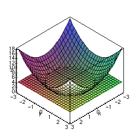
would be the solution of the equation x² + y² = 4.

There are several cases where it is important to be able to find the curves f(x, y) = C as the parameter C is varied, including the following

• On topographical maps, the function represents the altitude. By looking at the contours on such a map, you can determine how much climbing and descending you would have to do on a hike.
• Contours of pressure are often used by meteorologists as a way of locating fronts.
• Contours of temperature, velocity, field intensity, etc., are often used in science and engineering.

In fact, drawing the contours of a function z = f(x, y) in the xy plane is a way of representing a surface in two dimensions. That is, given the contour lines, you should be able to reconstruct the surface and vice-versa. There are several ways you can get Maple to generate the contours on a plot. One way is with the style=contour option when using the plot3d command as in the following example.

> plot3d(x^2 + y^2, x=-3..3, y=-3..3, style=contour, axes=boxed, labels=[x,y,z]);

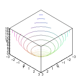
However, it is probably easier to generate the contours after you have used plot3d to render the surface, by using the Contour or Patch and contour options in the Style menu on the Maple 3D plotting window.

One thing to note is that Maple plots the contours right on the surface. Usually, by a contour plot, one means the projection of the contour curves onto the xy plane. To see this in Maple, just view the plot from above or below; that is, along the z axis. Alternatively, you can use the contourplot command which produces a 2D plot. This command is preferable unless you specifically want to see the contour lines plotted on the surface.

Examples
For this lab you will need to load the following two packages

> with(plots):
> with(plottools):

We first define a function of two variables

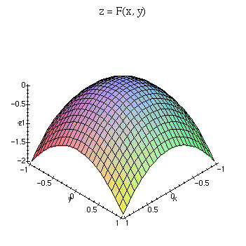
> F := (x,y) -> -(x^2 + y^2);

then use plot3d to see this 3-dimensional graph.

> plot3d(F(x,y), x=-1..1, y=-1..1, axes=framed, style=patch, title=`z = F(x, y)`, labels=[x,y,z]);

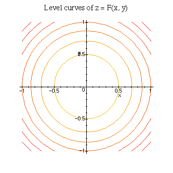
To see level curves of this function, we can use the contourplot command.

> contourplot(F(x,y), x=-1..1, y=-1..1, title=`Level curves of z = F(x, y)`);

If we want to view one specific level curve, that is, where z is fixed, we can specify that value in contourplot. In this example, we fix z = -0.5.

> contourplot(F(x,y), x=-1..1, y=-1..1, title=`F(x, y) = -0.5`, contours=[-0.5]);

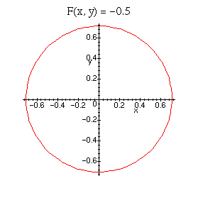
In order to display this curve and the plot of the original function on the same graph, we must convert the above 2D curve into 3D curve. (display only allows you to combine plots having the same dimension) We can do this by creating a function that transforms a 2D plot into a 3D one. Be sure to load the plottools package before issuing the following commands.

> level_plot := contourplot(F(x,y), x=-1..1, y=-1..1, color=black, thickness=2, contours=[-0.5]):
> surf_plot := plot3d(F(x,y), x=-1..1, y=-1..1):
> f := transform((x,y) -> [x,y,F(x,y)]):
> display({surf_plot, f(level_plot)}, axes=framed, title=`F(x, y) with level curve at z = -0.5`, labels=[x,y,z]);

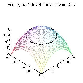
An alternative (and easier) way to accomplish the same result is to use contourplot3d instead of contourplot. This will produce a contour plot in 3D without requiring you to perform a conversion. The following commands are equivalent to those above.

> level_plot := contourplot3d(F(x,y), x=-1..1, y=-1..1, color=black, thickness=2, contours=[-0.5]):
> surf_plot := plot3d(F(x,y), x=-1..1, y=-1..1):
> display({surf_plot, level_plot}, axes=framed, title=`F(x, y) with level curve at z = -0.5`, labels=[x,y,z]);

Remember, you can get help at any time on a topic by using a question mark followed by the command name.

> ?contourplot

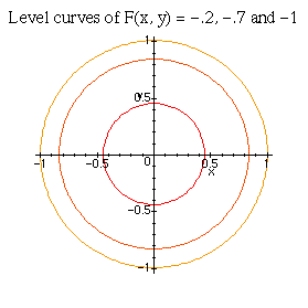
You should read through the help on contourplot by issuing the above command to find out how to utilize many of the options available. For example, you can either specify the number of equally spaced contour lines to display or choose exactly which values to use.

> contourplot(F(x,y), x=-1..1, y=-1..1, title=`Level curves of F(x, y) = -.2, -.7 and -1`, contours=[-0.2, -0.7, -1]);

Exercises

1. For each of the following functions,
   1. Plot the surface over the given rectangle.
   2. Plot several level curves in the rectangle.
   3. Plot the level curve of z through the given point P.
   1. z = x sin (y/2) + y sin 2x,       0 x 5, 0 y 5, P(3, 3)

   2. z = x² - y²,       -1 x 1, -1 y 1, P(1/2, 2/3)

   3. z = x² - y²,       1/2 x 3/2, 1/2 y 3/2, P(1, 1)

   4. z = -3x² + 3y² + 8xy + 10x + 20y + 25,       -3/2 x 1/2, -3 y -1, P(0, -5/3)

2. A hiker wants to forge a trail through a hilly region given by the relief function
   z = -3x² + 3y² + 8xy + 10x + 20y + 25

   The trail is assumed to lie at the constant height z = h.

   Determine if there exists a trail that connects the points P(5, 0) and Q(0, -5). If so, describe the shape of the trail and find the value of h.

   Plot the graph of the relief function and show the trail on this graph.

3. A spring is located at the point P in a hilly region with the relief function F. Assuming that the spring water flows along the -grad z vector at each point, find graphically the route of the brook initiated by the spring.

   In order to draw this, plot the level curve at the elevation of P, along with at least 4 other contours. Use your knowledge of calculus to trace the path of the brook (with a pencil on the printed plot).

   1. F := (x,y) -> exp(-x^2)*(1+cos(y));   P(1/2, 1/2)

   2. F := (x,y) -> exp(-x^2/9-y^2/9) + 2/3*exp(x-x^2/9+y/3-y^2/9-5/2) + exp(x-x^2/9-2*y/3-y^2/9-13/4)/2;   P(2, 1)

Back to the top